
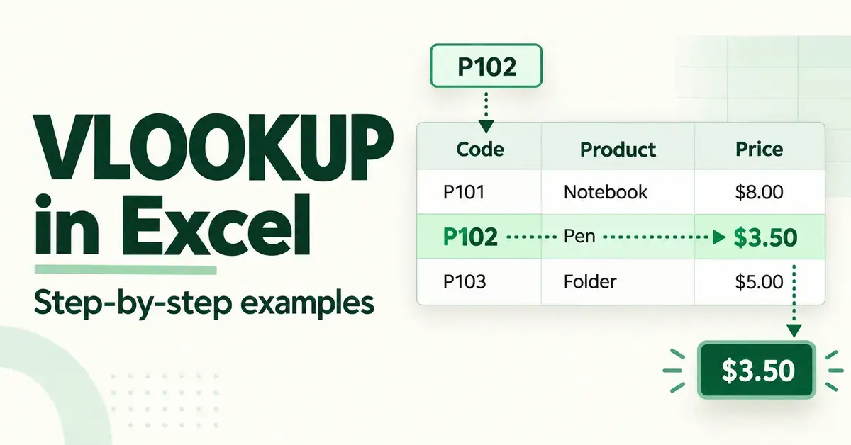
VLOOKUP is one of the most useful functions in Microsoft Excel: it looks up a value in the first column of a table and returns a matching value from another column in the same row. In plain terms, it answers questions like “what price goes with this product code?” or “what department is this employee in?” without you scrolling through thousands of rows by hand. This guide explains exactly how to use VLOOKUP in Excel, with the full syntax, several step-by-step worked examples, the most common errors and how to fix them, and when a newer function such as XLOOKUP is the better choice.
What does VLOOKUP do in Excel?
VLOOKUP stands for “vertical lookup.” It searches down the first column of a range for a value you specify, and when it finds a match it returns a value from a column further to the right in the same row. The “vertical” part matters: VLOOKUP scans down rows, not across columns. Its sister function, HLOOKUP, searches horizontally across the top row instead.
A typical use is matching two lists. Imagine a price list where column A holds product codes and column B holds prices. On another part of your sheet you type a product code, and VLOOKUP fetches the right price automatically. Because the lookup is driven by a formula, the answer updates the moment the underlying table changes, which makes VLOOKUP far safer and faster than copying values by hand.
Key Points
- What it does: VLOOKUP searches down the first column of a table and returns a value from another column in the same row.
- Syntax: =VLOOKUP(lookup_value, table_array, col_index_num, [range_lookup]).
- Exact match: add FALSE as the fourth argument for codes, names and IDs — this is the everyday setting.
- Approximate match: use TRUE only for sorted banded data such as tax brackets or grades.
- Biggest limit: VLOOKUP can only return values from columns to the right of the one it searches.
- Newer option: XLOOKUP (Excel 2021 and Microsoft 365) fixes most of VLOOKUP’s weaknesses.
The VLOOKUP syntax: the four arguments
The VLOOKUP formula always follows the same pattern: =VLOOKUP(lookup_value, table_array, col_index_num, [range_lookup]). Three arguments are required and the fourth is optional but almost always worth including. Here is what each one means.
lookup_value — what you are searching for
This is the value Excel hunts for in the first column of your table. It can be a number, a piece of text, a date, or a reference to a cell that holds one of those (for example A2). Whatever you choose must sit in the left-most column of the range you point VLOOKUP at, because VLOOKUP only ever searches that first column.
table_array — the range to search
This is the block of cells containing both the column you are searching and the column holding the answer you want back. For example $D$2:$F$500 covers columns D, E and F. The dollar signs lock the range so it does not shift when you copy the formula down a list — a small habit that prevents a lot of broken results. You can also point VLOOKUP at a named range or an Excel Table, which keeps formulas readable.
col_index_num — which column holds the answer
This is a number telling Excel which column of the table_array to return a value from, counting from the left. The first (left-most) column of the range is 1, the next is 2, and so on. If your table_array is D2:F500 and the answer lives in column F, the index number is 3, because F is the third column inside that range — not because F is the sixth column of the worksheet. Counting from the worksheet instead of from the range is one of the most common beginner mistakes.
range_lookup — exact or approximate match
This optional argument decides how fussy VLOOKUP is. Set it to FALSE (or 0) for an exact match, and set it to TRUE (or 1) for an approximate match. If you leave it out entirely, Excel assumes TRUE, which surprises many people. For the vast majority of real-world lookups — product codes, names, IDs — you want FALSE, so make a habit of typing it every time.
How to use VLOOKUP: a step-by-step example
Suppose you have a staff list. Column A holds employee IDs, column B holds names and column C holds departments, filling rows 2 to 100. You want to type an ID in cell E2 and have Excel return that person’s department in F2.
- Step 1. Click the cell where you want the answer (F2) and type =VLOOKUP(.
- Step 2. Click cell E2, or type E2, as your lookup_value, then type a comma. This is the ID you are searching for.
- Step 3. Select the table that contains both the IDs and the departments — here $A$2:$C$100 — then type a comma. The IDs must be in the first column of this range.
- Step 4. Type the column index. Departments are in column C, which is the third column of the range, so type 3 followed by a comma.
- Step 5. Type FALSE to force an exact match, then close the bracket. The finished formula reads =VLOOKUP(E2,$A$2:$C$100,3,FALSE).
- Step 6. Press Enter. Type a real employee ID into E2 and the matching department appears in F2 instantly.
That single formula now works for any ID you enter. Because the range is locked with dollar signs, you can copy the formula down a whole column of IDs and each row looks up its own answer.
Exact match versus approximate match, with examples
The range_lookup argument is where VLOOKUP causes the most confusion, so it is worth seeing both modes in action.
Exact match (FALSE): the everyday choice
Exact match returns a value only when it finds the lookup_value spelled or numbered precisely. Using the staff example, =VLOOKUP(“E-104”,$A$2:$C$100,2,FALSE) returns the name tied to ID E-104 and nothing else. If that ID does not exist, VLOOKUP returns an #N/A error rather than guessing. This is exactly what you want for codes, SKUs, names and anything where a near-miss would be wrong.
Approximate match (TRUE): for banded ranges
Approximate match is designed for lookups into graduated bands, such as tax brackets, commission tiers or grade boundaries. Instead of an exact hit, VLOOKUP finds the largest value that is less than or equal to your lookup_value. The crucial rule: the first column of your table must be sorted in ascending order, or the results will be wrong without any error warning.
For example, say a grade table lists score thresholds 0, 50, 65, 80 in column A and grades F, C, B, A in column B. The formula =VLOOKUP(72,$A$2:$B$5,2,TRUE) returns “B”, because 72 falls into the band that starts at 65. Because you are matching a number to a range rather than to an exact value, TRUE (or a blank fourth argument) is correct here — one of the few times leaving range_lookup out is acceptable.
Using VLOOKUP across different sheets and workbooks
VLOOKUP is not limited to a single sheet. To pull data from another worksheet, include the sheet name in the table_array, separated by an exclamation mark: =VLOOKUP(A2,Prices!$A$2:$C$500,3,FALSE) looks up the value from cell A2 inside a sheet called “Prices.” If the sheet name contains spaces, Excel wraps it in single quotes, for example =’Price List’!$A$2:$C$500.
You can even reference another workbook by including the file name in square brackets, though lookups that point at a closed external file can slow a workbook down and break if the other file moves. For shared or long-lived spreadsheets it is usually cleaner to copy the reference data into the same workbook, or to use Power Query to pull it in.
Common VLOOKUP errors and how to fix them
When VLOOKUP returns an error, the message itself tells you what went wrong. These are the ones you will meet most often.
- #N/A (value not found). This is the most common error and simply means VLOOKUP could not find your lookup_value. Check for typos, and for invisible leading or trailing spaces, which you can strip with the TRIM function. Also make sure the lookup value really is in the first column of the range. In approximate-match mode, #N/A can also mean the lookup value is smaller than everything in the column, or that the column is not sorted ascending.
- #REF! (bad column number). This appears when col_index_num is larger than the number of columns in your table_array — for example asking for column 4 of a three-column range. Fix the index number, or widen the range.
- #VALUE! (invalid argument). This usually means col_index_num is less than 1, or part of the formula is broken. Column numbers must start at 1.
- #NAME? (misspelled function). Normally a typing slip such as “VLOKUP” or a missing quotation mark around text. Check the spelling of the function and any text values.
- The wrong value comes back. No error, but the answer is clearly incorrect. The usual culprit is a forgotten range_lookup — Excel defaulted to approximate match and returned the nearest band. Add FALSE for an exact match.
The limitations of VLOOKUP
VLOOKUP is powerful, but it has real constraints that are worth understanding before you build a big spreadsheet around it.
- It can only look to the right. The return column must sit to the right of the lookup column. VLOOKUP cannot fetch a value from a column to the left of the one it searches, which is its single biggest weakness.
- It breaks when you insert columns. The col_index_num is a fixed number. If you insert a new column inside the table, the answer column shifts but the formula still points at the old position, silently returning the wrong data.
- It returns only the first match. If a value appears more than once in the first column, VLOOKUP always returns the first one it meets from the top, ignoring any later matches.
- Approximate match needs sorted data. As covered above, TRUE mode only works correctly when the first column is sorted in ascending order.
If you work with large, data-heavy spreadsheets regularly, it is worth reading more widely on Excel data management so these limitations do not catch you out mid-project.
VLOOKUP versus XLOOKUP and INDEX/MATCH
VLOOKUP is not the only lookup tool in Excel, and in newer versions it is no longer the best one. Two alternatives solve its main weaknesses.
XLOOKUP was introduced in Excel 2021 and Microsoft 365 (and works in Excel for the web). It defaults to an exact match, can look in any direction including to the left, follows the answer column automatically when you insert columns, and has a built-in option to display a friendly message instead of #N/A. The catch is that XLOOKUP does not exist in Excel 2019 or earlier, so if you share files with people on older versions, VLOOKUP remains the compatible choice.
INDEX/MATCH combines two older functions to achieve the same lookup in any direction, and it works in every version of Excel. It is more flexible than VLOOKUP but harder to read, which is why many people now jump straight from VLOOKUP to XLOOKUP. The table below sums up the trade-offs.
VLOOKUP vs XLOOKUP vs INDEX/MATCH
| Feature | VLOOKUP | XLOOKUP | INDEX/MATCH |
|---|---|---|---|
| Available in | All Excel versions | Excel 2021, Microsoft 365, Excel for the web | All Excel versions |
| Default match type | Approximate (TRUE) | Exact | Exact (with MATCH 0) |
| Can look left | No | Yes | Yes |
| Survives inserted columns | No (fixed column number) | Yes | Yes |
| Built-in “not found” message | No | Yes (if_not_found) | No |
| Ease for beginners | Easy | Easy | Harder to read |
Does VLOOKUP work outside Microsoft Excel?
Yes. VLOOKUP is a standard spreadsheet function, and it behaves almost identically in the free office suites and in cloud spreadsheets. LibreOffice Calc and Apache OpenOffice Calc both include VLOOKUP with the same arguments, so formulas built in Excel usually carry straight across — useful if you are moving to a free suite like LibreOffice or OpenOffice. Google Sheets also supports VLOOKUP, with the small difference that it uses semicolons instead of commas in some regional settings; our Google Sheets formulas guide walks through VLOOKUP and its Sheets-specific quirks. If you need Excel itself, the function is included in every desktop and web edition, which you can read about in our overview of Microsoft 365 Business plans.
Common mistakes to avoid
Most VLOOKUP problems come down to a handful of avoidable habits. Keep these in mind and the function will behave predictably.
- Forgetting FALSE. Leaving out the fourth argument lets Excel default to approximate match, which quietly returns the wrong value on unsorted data. Type FALSE for every exact lookup.
- Not locking the range. Without dollar signs ($A$2:$C$100), the table_array drifts as you copy the formula down, so lower rows search the wrong cells.
- Counting columns from the worksheet. The col_index_num counts from the first column of your range, not from column A of the sheet.
- Mismatched data types. A lookup can fail when the ID in your lookup cell is stored as text but the ID in the table is stored as a number (or vice versa). Make both the same format.
- Hidden spaces. Data imported from other systems often carries trailing spaces that break an exact match. TRIM or Find & Replace will clean them.
- Searching a column that is not on the left. Remember VLOOKUP looks only to the right; if your answer is to the left, switch to XLOOKUP or INDEX/MATCH rather than rearranging your data.
For a broader look at building reliable, formula-driven sheets — from lookups to summaries and charts — our wider spreadsheet template guides show the same principles applied to everyday planning.
Sources
Frequently Asked Questions (FAQ)
What is the simplest way to write a VLOOKUP formula?
Type =VLOOKUP( then give it four things in order: the value you are looking for, the table to search, the number of the column that holds the answer counting from the left of that table, and FALSE for an exact match. For example, =VLOOKUP(E2,$A$2:$C$100,3,FALSE) looks up the value in E2 and returns the matching entry from the third column of the range.
Why does my VLOOKUP return #N/A?
The #N/A error means Excel could not find your lookup value. The usual causes are a typo, hidden spaces around the text, the lookup value not being in the first column of the range, or the two values being stored in different formats such as text versus number. In approximate-match mode it can also appear when the first column is not sorted in ascending order.
What is the difference between TRUE and FALSE in VLOOKUP?
FALSE (or 0) forces an exact match and is what you want for codes, names and IDs. TRUE (or 1) allows an approximate match that finds the largest value less than or equal to your lookup value, which suits banded data like tax brackets or grades, but it only works if the first column is sorted ascending. If you omit the argument, Excel assumes TRUE.
Can VLOOKUP look to the left?
No. VLOOKUP can only return a value from a column to the right of the one it searches. If the answer you need sits to the left of your lookup column, use XLOOKUP (in Excel 2021 or Microsoft 365) or the INDEX/MATCH combination, both of which can look in any direction.
Should I use VLOOKUP or XLOOKUP?
Use XLOOKUP if you have Excel 2021, Microsoft 365 or Excel for the web, because it defaults to exact match, can look in any direction and handles errors more gracefully. Stick with VLOOKUP when you need the file to work in Excel 2019 or earlier, since XLOOKUP is not available in those older versions.
