
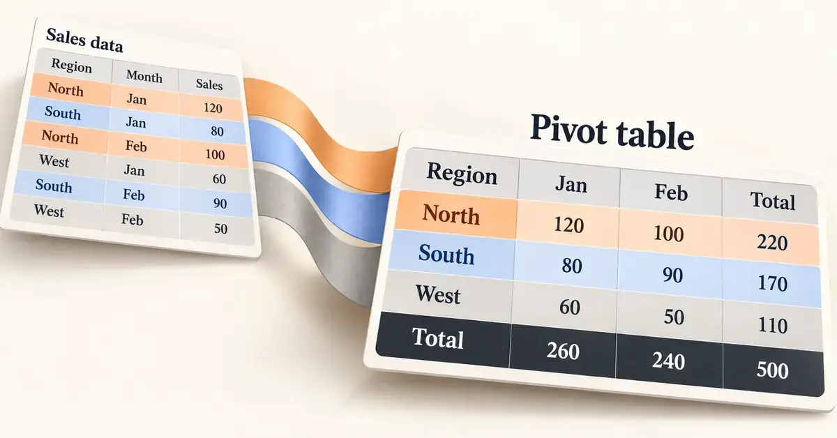
A pivot table in Google Sheets is a tool that summarises a large table of raw data into a short, readable report — totals, counts and averages grouped the way you want — without you writing a single formula. If you have ever stared at hundreds of rows of sales, survey answers or expenses and wondered what the numbers actually add up to, a pivot table answers that question in seconds. This guide explains what pivot tables are, walks through building one step by step, and covers summarising, filtering, calculated fields and the mistakes that trip up beginners.
Everything below was checked against Google’s own Sheets documentation and reflects the editor as it works in late 2026, including the updated calculated-fields editor that rolled out in September 2026.
What is a pivot table in Google Sheets?
A pivot table is an interactive summary of a data range. You feed it a flat table — one row per record, one column per attribute — and it groups those records and calculates a figure for each group. The word “pivot” refers to how you can rotate the same data: put product categories down the side one minute, swing them across the top the next, and the totals rearrange instantly.
A simple example: imagine a sheet with one row per order, holding the columns Date, Region, Product and Amount. A pivot table can turn that into “total sales by region,” “average order value by product,” or “number of orders per month” — each as a tidy grid. Change the source data and the pivot table updates on its own.
Pivot tables differ from ordinary spreadsheet functions. A formula such as SUMIF answers one fixed question in one cell; a pivot table builds a whole cross-tabulated report you can reshape by dragging fields. If you are comfortable with Google Sheets formulas but find yourself writing dozens of SUMIFs to slice the same dataset, a pivot table usually does the job faster and with fewer errors.
Key Points
- What it does: A pivot table summarises a large data range into grouped totals, counts and averages — no formulas required.
- How to start: Select your data, then choose Insert > Pivot table and build it in the editor panel on the right.
- The four sections: Rows and Columns group the data; Values do the maths; Filters narrow it down.
- Summarise and reshape: Use Summarize by (SUM, COUNT, AVERAGE and more) and Show as to switch between totals and percentages.
- Cost: Free with any Google account; best built on a desktop browser.
What you need before you start
You need remarkably little. Pivot tables are a built-in feature of Google Sheets, so there is nothing to install or pay for.
- A free Google account. Google Sheets is free to use with a personal Google account, and the pivot-table feature is included in both personal and paid Google Workspace plans.
- A web browser or the Sheets app. The full editor works best on a desktop browser such as Chrome, Edge, Firefox or Safari.
- Clean source data. Each column should have a single header row at the top, no blank rows or columns inside the data, and consistent values in each column (dates stored as dates, numbers as numbers). Messy source data is the single biggest cause of confusing pivot tables.
If your data currently lives in a CSV export from another program, import it first — our guide on how to open a CSV file in Sheets, Excel and Calc covers that cleanly.
How to create a pivot table in Google Sheets step by step
Here is the complete process from a raw table to a finished summary. The whole thing takes under a minute once you know where the buttons are.
Step 1 — Prepare and select your data
Open your spreadsheet and click any single cell inside your data; Google Sheets will usually detect the full range automatically. If you prefer to be precise, highlight the exact range you want, including the header row. Make sure every column has a header, because those headers become the field names in the pivot table editor.
Step 2 — Insert the pivot table
Go to the Insert menu and choose Pivot table. A small dialog asks whether to place the pivot table in a New sheet or an Existing sheet. A new sheet keeps things uncluttered and is the safer choice while you are learning. Click Create, and Sheets opens an empty pivot table with an editor panel on the right-hand side.
Step 3 — Add rows and columns
The editor has four sections: Rows, Columns, Values and Filters. Next to Rows, click Add and pick the field you want listed down the left side — Region, for instance. Each unique value in that field becomes its own row. To break the data down a second way, click Add next to Columns and choose another field, such as Product; its values spread across the top, creating a grid.
Step 4 — Add values and choose how to summarise
This is where the numbers appear. Next to Values, click Add and choose the field you want to calculate, such as Amount. By default Sheets totals it with SUM, but you can change that using the Summarize by menu (covered in the next section). You can add more than one value — for example, both the sum of sales and the count of orders — and they will sit side by side.
Step 5 — Filter and sort
To narrow the report, click Add next to Filters and choose a field, then filter by condition (such as “greater than” or “text contains”) or by ticking the values to show. To reorder the results, use the Order and Sort by controls under any Rows or Columns field. Your pivot table is now complete, and it will refresh automatically whenever the source cells change.
How to summarise data: Summarize by and Show as
The Summarize by menu controls the maths applied to each value field. Click the field under Values and open the menu to switch between the common options:
- SUM — adds the numbers up (the default for numeric fields).
- COUNT and COUNTA — count numeric entries, or all non-empty entries.
- COUNTUNIQUE — counts distinct values, useful for “how many different customers.”
- AVERAGE, MAX, MIN and MEDIAN — the usual statistical summaries.
- STDEV and VAR — spread and variance for more advanced analysis.
Next to that sits Show as, which changes how each figure is displayed rather than how it is calculated. Instead of raw totals you can show each cell as a % of grand total, % of row or % of column — the quickest way to turn absolute numbers into percentages without a single extra formula. To add one, click the word Default under the value field and pick the option you want.
Using filters, grouping and slicers
Filters placed inside the pivot table editor only affect that one pivot table. If you want controls that filter the pivot table and any charts beside it on the same sheet, add a slicer from the Data > Add a slicer menu — it appears as an on-sheet drop-down button that anyone viewing the sheet can click. Slicers are the more presentation-friendly option for dashboards.
You can also group rows to collapse detail. Right-click a row or column header to group items manually, by numeric intervals, or by date and time periods such as month, quarter or year — a tidy way to roll daily records up into monthly figures. The same right-click menu ungroups them again. This pairs well with techniques like conditional formatting, which you can apply to the finished pivot output to highlight the largest or smallest values.
Calculated fields: creating your own metrics
A calculated field is a column you invent inside the pivot table from the fields already there. The classic example is profit: if your data has Sales and Cost columns, a calculated field of Sales - Cost gives profit per group without touching the source data.
To add one, click Edit under the pivot table, then Add next to Values and choose Calculated field. As of the update Google rolled out in September 2026, calculated fields open in a dedicated editor window rather than a cramped sidebar card. The new editor gives you menus for selecting column names — so you no longer have to type field names exactly — and it checks your syntax live, flagging errors before the change is applied. A green tick means the formula is valid; a red mark means something needs fixing. If a field name contains spaces, wrap it in quotation marks inside the formula. The techniques will feel familiar if you already use lookup functions like VLOOKUP in Google Sheets.
Suggested pivot tables
When you insert a pivot table, the editor panel often shows ready-made layouts under a Suggested heading — “Sum of Amount for each Region,” for example. Clicking one builds that report instantly, which is a fast way to explore unfamiliar data. Google may also insert a high-confidence suggestion automatically. If you prefer to build every table by hand, turn the suggestions off under Tools > Suggestion controls by disabling Enable Pivot table suggestions.
Editing, refreshing and deleting a pivot table
To change a finished pivot table, click any cell in it and the editor panel reopens; from there you can drag fields between sections, remove them, or use Clear all to start over. The Select data range control lets you point the table at a different or expanded source range — useful when you add new rows below your original data.
Pivot tables refresh themselves whenever the source cells change, so there is no manual “refresh” button to hunt for. If new data does not appear, it is almost always because the new rows fall outside the defined source range. To see the underlying records behind any single figure, double-click that cell and Sheets opens a new tab listing those source rows. To delete the pivot table, simply select it and clear the cells, or delete the sheet it lives on.
Can you make a pivot table on the mobile app?
The Google Sheets apps for Android and iOS can open and view spreadsheets that contain pivot tables, and the tables keep working when the source data changes. However, the full pivot-table editor — dragging fields, choosing summaries and building calculated fields — is designed for the desktop browser and is awkward or unavailable on a small screen. For anything beyond viewing, use a computer. If you need a spreadsheet on the go, settings like Google Sheets dark mode make the mobile app easier on the eyes for reading reports.
Pivot tables in Google Sheets vs Excel vs Calc
Pivot tables are not unique to Google Sheets. Microsoft Excel pioneered the feature, and the free OpenDocument suites include their own version. The core idea is identical everywhere; the differences are in polish, collaboration and advanced options.
Comparison
| Feature | Google Sheets | Microsoft Excel | LibreOffice / OpenOffice Calc |
|---|---|---|---|
| Cost | Free with a Google account | Paid (Microsoft 365 or Office) | Free and open-source |
| Where it runs | Web browser; limited on mobile | Desktop, web and mobile apps | Desktop (Windows, Mac, Linux) |
| Name of the feature | Pivot table | PivotTable | Pivot Table (OpenOffice calls it DataPilot) |
| Calculated fields | Yes, with a 2026 formula editor | Yes, long-established | Yes |
| Live collaboration | Yes, built in | Yes, via the cloud | No real-time co-editing |
| Official page | sheets.google.com | microsoft.com/excel | libreoffice.org / openoffice.org |
If you mostly work in a free desktop suite, our beginner’s guide to OpenOffice Calc explains its DataPilot approach to the same task, and files save in the open ODS spreadsheet format that Google Sheets can import and export.
Common mistakes to avoid
Most pivot-table frustration comes from a handful of avoidable issues rather than the feature itself.
- Missing or merged headers. Every column needs a single, unique header. Merged cells and blank header cells confuse the editor and produce fields with no name.
- Blank rows inside the data. An empty row can cut your source range short, so part of your data silently never reaches the pivot table.
- Numbers stored as text. If amounts were imported as text, SUM returns zero or nothing. Check that numeric columns are right-aligned and formatted as numbers.
- A source range that never grows. When you add new records, they only appear if they fall inside the defined range. Either include whole columns in the range or update it with Select data range.
- Over-filtering and forgetting. It is easy to leave a filter on and then wonder why totals look low. Check the Filters section before trusting a surprising number.
- Editing the pivot output directly. You cannot type over pivot-table cells; change the data or the editor, not the result grid.
Who are pivot tables for?
Pivot tables suit anyone who needs to summarise more data than they can read at a glance. Small-business owners use them for sales and expense reporting; teachers and researchers tally survey and test results; club treasurers track subscriptions; and office teams turn raw exports into monthly figures for a meeting. They pair naturally with other reporting tools — a tidy data-entry sheet using a drop-down list feeds clean data straight into a pivot table. You do not need to be an analyst: if you can open a menu and drag a field name, you can build one.
Sources
Frequently Asked Questions (FAQ)
Is the pivot table feature in Google Sheets free?
Yes. Pivot tables are a standard part of Google Sheets and cost nothing. They are available with a free personal Google account as well as with paid Google Workspace plans, and there is nothing extra to install or enable.
Why is my pivot table not showing new data?
Pivot tables refresh automatically when the source cells change, so if new rows are not appearing, they almost certainly fall outside the table’s defined source range. Click the pivot table, open the editor and use the Select data range control to extend the range — or define the source as whole columns so future rows are always included.
Can I create a pivot table on the Google Sheets mobile app?
You can open and view spreadsheets containing pivot tables on the Android and iOS apps, and they stay accurate as data changes. Building or heavily editing a pivot table, though, is designed for the desktop browser, where the full editor panel is available. For anything beyond viewing, use a computer.
What is the difference between a pivot table and a SUMIF formula?
A SUMIF formula answers one fixed question in a single cell, while a pivot table builds a whole cross-tabulated report you can reshape by dragging fields. If you only need one total, a formula is fine; if you need to slice the same dataset many ways, a pivot table is faster and less error-prone.
How do I add a percentage column to a pivot table?
Click the value field in the editor, then open the Show as menu (it says Default by default) and choose % of grand total, % of row or % of column. The figures are redisplayed as percentages without any extra formula or calculated field.
