
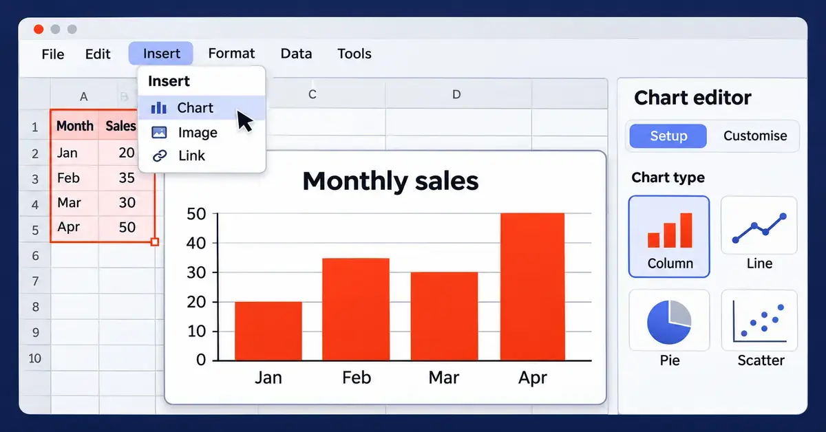
To make a graph in Google Sheets, select the cells that hold your data, open the Insert menu and choose Chart. Google Sheets instantly draws a chart and opens a Chart editor on the right, where you can change the chart type and adjust how everything looks. That is the whole workflow in one sentence — but choosing the right chart and tidying it up is where a good graph is won or lost. This guide walks through every step, explains which chart type suits which data, and covers the mistakes that trip up most beginners.
Key Points
- Fastest route: select your data, then Insert > Chart. Google Sheets draws a chart and opens the Chart editor.
- Two tabs: the Setup tab sets the chart type and data range; the Customise tab controls titles, colours, legend and axes.
- Match type to question: columns/bars compare categories, lines/areas show trends over time, pies show parts of a whole, scatter shows relationships.
- Live updates: charts redraw automatically when the source cells change; extend the data range when you add new rows.
- Reuse anywhere: copy a chart into Docs or Slides, or download it as a PNG, PDF or SVG.
What is a chart in Google Sheets, and when should you use one?
A chart (also called a graph) is a visual picture of numbers in your spreadsheet — bars, lines, slices or dots that make a pattern obvious at a glance. In Google Sheets the words “chart” and “graph” mean the same thing; the menus and the Chart editor all say “chart”.
Reach for a chart whenever a table of numbers is hard to read. A column of monthly sales figures tells you little until you see them climb or fall in a line chart. Use a graph to compare categories, show a trend over time, reveal how a total breaks into parts, or spot an outlier. If the data is small or the exact figures matter more than the pattern, a plain table is often clearer — a chart is for showing shape and relationship, not for looking up precise values.
How to set up your data before you make a graph
A good chart starts with tidy data, so lay out your numbers before you insert anything. A few rules make every chart cleaner:
- Use one row of headers. Put a short label at the top of each column (for example “Month” and “Sales”). Google Sheets reads these as the names for your axis and legend.
- Keep categories in the first column. The left-most column usually becomes the horizontal axis — months, products or regions.
- One value per cell, no blanks. Empty cells leave gaps in the graph. If a value is genuinely zero, type 0.
- Keep the numbers as numbers. A figure stored as text (for example “1,200 kg” with the unit typed in) will not plot. Store the number alone and format the cell to show units.
If your raw data is messy or very large, summarise it first. A pivot table in Google Sheets can collapse thousands of rows into a tidy summary that charts beautifully, and Google Sheets formulas such as SUM or AVERAGE let you build the totals you actually want to plot.
How to make a graph in Google Sheets, step by step
Here is the full process on a computer, from a blank chart to a finished graph.
Step 1: Select your data
Click and drag to highlight the cells you want to chart, including the header row and label column. To select ranges that are not next to each other, hold Ctrl (or Cmd on a Mac) while you drag over each block. You can also click any single cell inside a tidy block and Google Sheets will guess the full range for you.
Step 2: Insert the chart
Open the Insert menu at the top and choose Chart. Google Sheets adds a chart to the sheet straight away and picks a type it thinks fits your data — often a column or line chart. The Chart editor opens on the right.
Step 3: Choose the chart type in the Setup tab
In the Chart editor, the Setup tab controls what the chart shows. Open the Chart type drop-down to switch to any other type. The list starts with a Suggested group — types Google thinks suit your selection — followed by every type grouped by family (line, area, column, bar, pie, scatter, map and others).
Step 4: Check the data range and headers
Still in the Setup tab, confirm the Data range is correct; click the small grid icon to reselect cells or use Add another range to fold in more data. Tick Use row 1 as headers so your labels appear on the chart, and use Switch rows / columns if the axis and legend are the wrong way round.
Step 5: Customise the look
Switch to the Customise tab to style the graph — titles, colours, legend, axes and gridlines. The next section covers this in detail.
Step 6: Place and save
Close the editor when you are done. Your chart is saved automatically with the spreadsheet. Drag it to move it, or drag the blue corner handles to resize it. Because the chart is linked to the cells, it updates on its own whenever you change the underlying numbers.
Which chart type should you choose?
The right chart type depends on the question you want the graph to answer. Google Sheets offers more than two dozen types, but a handful cover almost every everyday need.
Column and bar charts — comparing categories
Column charts (vertical) and bar charts (horizontal) compare values across categories, such as sales per product or visitors per region. Use a horizontal bar chart when category names are long, so the labels have room to read. Stacked versions show how a total splits into parts.
Line and area charts — trends over time
A line chart is the standard choice for showing how a value changes over time — daily temperatures, monthly revenue, weekly sign-ups. An area chart is a line chart with the space beneath filled in, which helps when you want to emphasise volume or stack several series.
Pie and doughnut charts — parts of a whole
A pie chart shows how one total divides into slices, such as market share or budget split. Keep it to a handful of slices — more than about eight becomes unreadable — and avoid pies when the slices are close in size, because the eye cannot judge small differences in angle.
Scatter charts — relationships between two numbers
A scatter chart plots one number against another to reveal a relationship, for example advertising spend against sales. Each point is one observation; a cloud that trends upward suggests the two move together.
Combo charts and specialised types
A combo chart layers two types together — typically columns plus a line — so you can show, say, monthly revenue as bars with a profit-margin line on top. For niche needs, Google Sheets also includes histograms, geo/map charts, waterfall, radar, gauge, organisational, tree map, candlestick (stock) and annotated-timeline charts. If you need a project schedule rather than a data chart, see our Gantt chart template guide.
Chart Types at a Glance
| Chart type | Best for | Example |
|---|---|---|
| Column / Bar | Comparing values across categories | Sales by product |
| Line | A trend over time | Monthly revenue |
| Area | Trend plus volume, or stacked series | Website traffic by channel |
| Pie / Doughnut | How a total splits into parts | Budget share |
| Scatter | Relationship between two numbers | Ad spend vs sales |
| Combo | Two measures together (bars + line) | Revenue with margin line |
| Geo / Map | Values by country or region | Customers by region |
| Histogram | How often values fall in each range | Distribution of order sizes |
How to customise your chart
Every styling control lives in the Customise tab of the Chart editor (double-click a chart to reopen the editor). The sections you will use most are:
- Chart style — background colour, overall font and border, plus options that vary by chart type.
- Chart & axis titles — pick the title you want from the drop-down (chart title, subtitle, horizontal or vertical axis title), type the text and set its font, size and colour.
- Series — recolour individual data series, add data labels that print the value on each bar or point, and add trendlines.
- Legend — move the legend to the top, bottom, left, right or off, and change its font.
- Horizontal / vertical axis — set the label font, reverse the order, or change the scale (handy to force a value axis to start at zero).
- Gridlines and ticks — adjust how many gridlines show and their spacing.
To restyle just one bar or slice, right-click it and choose Format data point, then pick a colour. Keep the palette simple: one accent colour for the series that matters and a neutral grey for the rest reads far better than a rainbow. If you work in a dimmed interface, our guide to dark mode in Google Sheets explains how the editor behaves.
How to edit, move, copy and download a chart
Once a chart exists you can reuse it anywhere:
- Edit — double-click the chart to reopen the Chart editor, or click it once and use the three-dot menu in its top-right corner.
- Move or resize — drag the chart to reposition it, or drag the corner handles to change its size.
- Copy into Docs or Slides — use the three-dot menu, choose Copy chart, then paste into a Google Doc or Slides file. Keep it linked so it refreshes when the sheet changes, or unlinked to freeze a snapshot.
- Download — the same three-dot menu offers Download as a PNG image, PDF or scalable SVG for use outside Google.
- Move to its own tab — choose Move to own sheet to give the chart a full-screen tab, useful for dashboards.
How to make a graph in the Google Sheets mobile app
You can build a basic chart on the Google Sheets app for Android, iPhone and iPad, though with fewer options than the desktop. Open the spreadsheet, tap and drag the blue selection handles to highlight your data, tap the + (Insert) button and choose Chart. Tap the chart to edit it, where you can change the type, title and colours. To widen the data range later, select the chart, open its editor and adjust the range. Fine styling — detailed axis scales, trendlines, per-point colours — is easier to finish on a computer, so many people rough out a chart on mobile and polish it later in a browser.
Common mistakes to avoid
A few errors show up again and again when beginners make graphs in Google Sheets:
- Picking the wrong chart type. A pie chart for a trend over time, or a line chart for unrelated categories, misleads readers. Match the type to the question (trend, comparison or share).
- Too many pie slices. Beyond roughly eight categories a pie becomes a muddle; group small items into “Other” or switch to a bar chart.
- A value axis that does not start at zero. For bar and column charts a non-zero baseline exaggerates differences. Line charts can sometimes start higher, but say so.
- Numbers stored as text. If a series refuses to plot, check the cells are real numbers, not text with units typed in.
- Forgetting to extend the data range. Adding new rows does not always pull them into an existing chart — reopen the editor and update the range.
- Overcrowding. Chart junk — heavy gridlines, drop shadows, five colours — hides the message. Strip back to the data and one or two labels.
Google Sheets charts versus other free tools
Google Sheets charting is free, browser-based and updates live as data changes, which makes it ideal for shared dashboards and quick reports. Microsoft Excel offers deeper charting (more types, finer control and PivotCharts) but its full feature set needs a paid licence. If you prefer an offline, fully free desktop spreadsheet, the chart tools in OpenOffice Calc and in LibreOffice Calc cover the same common chart types without any subscription, and both can open data you export from Google. When you move data between apps, our guide on how to open a CSV file helps you keep the numbers intact so the charts rebuild cleanly.
Who should use Google Sheets for graphs?
Google Sheets suits anyone who wants to turn data into a visual quickly and share it — students, small-business owners, teachers, community groups and teams who collaborate online. It is especially good when several people edit the same data and everyone needs the chart to stay current. If you need publication-grade statistical graphics or very large datasets, a dedicated data tool will serve better, but for everyday reporting the built-in charts are more than enough.
Sources
Frequently Asked Questions (FAQ)
How do I make a simple bar graph in Google Sheets?
Highlight your category labels and their values, open the Insert menu and choose Chart. In the Chart editor on the right, open the Chart type drop-down and pick a column chart (vertical bars) or bar chart (horizontal bars). Then use the Customise tab to add a title and tidy the colours.
Why is my chart not showing any data?
The usual causes are numbers stored as text, blank cells breaking the series, or a data range that does not cover your figures. Check that the cells contain plain numbers, fill genuine zeros with 0, and reopen the Chart editor to confirm the Data range includes the rows and columns you expect.
Do Google Sheets charts update automatically?
Yes. A chart is linked to the cells it was built from, so when you change a value the chart redraws on its own. The exception is new rows or columns added outside the original range — for those you reopen the Chart editor and extend the Data range to include them.
Can I make a graph in the Google Sheets mobile app?
Yes. Select your data, tap the plus (Insert) button and choose Chart, then tap the chart to change its type, title and colours. The mobile app offers fewer styling options than the desktop version, so detailed customising is easier to finish in a web browser.
How do I move a Google Sheets chart into Google Docs or Slides?
Click the chart, open its three-dot menu and choose Copy chart, then paste it into your Google Doc or Slides file. You can keep it linked so it refreshes when the spreadsheet changes, or paste it unlinked to freeze the current version as a static image.
